Predicting Data Scientist Salaries Using Logistic Regression

Predicting Data Scientist Salaries Using Logistic Regression

Scenario involves being a data scientist contracted by a firm that is rapidly expanding. Looking for new data scientist is vital for the expansion. Management thinks the best way to gauge salary amounts is to take a look at what industry factors influence the pay scale for data scientist. The jupyter code can be found here.. This was done as a group project with JP Freeley, Jesse Sanford, and Kristen Su.

The following steps are taken in this analysis:

1. Scraping Indeed, Glassdoor, and Cost of Living index
2. Combining into separate Data Frames
3. Cleaning/Tidying Data
4. Plotting/Normalizing
5. Regressions

The cities scraped for this project were: Atlanta, Austin, Boston, Dallas, Detroit, Houston, Kansas City, Los Angeles, Minneapolis, Nashville, San Francisco, San Jose, and Washington DC.

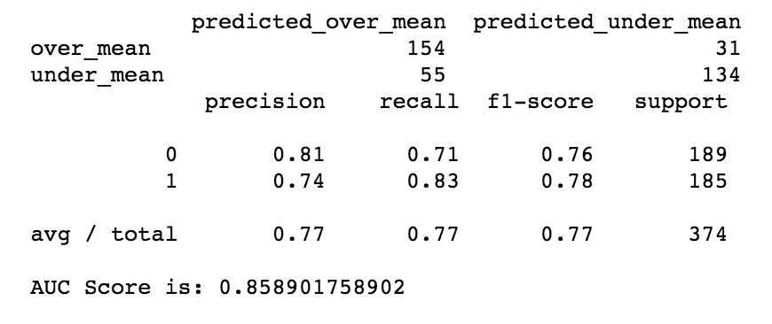
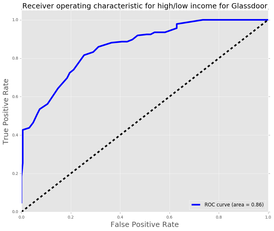
The process was to perform a regression on glassdoor salaries, and then use the model to predict the data from Indeed. Findings from the regression found that incorporating Cost of Living Index with the median Salary found on glassdoor, with binning the titles into Entry-level, Mid-level, and Senior Level bins, and creating dummy variables for each city gave an AUC score of 0.86 (with 1 being perfect) and F1 score of 0.77. The AUC score is a metric that analyzes the relationship between false positives and True positives while running a classification regression. The F1 score looks at the accuracy of the model.

What does this mean? Well, normalizing for cost of living, the salary is dependent on experience level and location. As the demand for data scientist is increasing, to attract the brightest minds, a company might be more inclined to overpay if the company is located outside of Bay Area, New York, Washington DC, and Boston (all had negative coefficients).

Scraping Indeed, Glassdoor, and Cost of Living Index

Scraping Indeed

The scraper code used to pull informat from indeed, can be found in the jupiter notebook located here.

Glassdoor

The scraper code used to pull informat from Glassdoor, can be found here.. This code was forked from here.

Cost of Living Index

The code to scrape for Cost of Living index from www.expatistan.com.

Cleaning & Tidying the DataFrames

Extensive cleaning was performed to convert salaries into low salary, high salary and median salary, as well cleaning cities and titles, including binning into entry, mid, and senior-level bins. The jupyter notebook contains all the code for the cleaning.

Visualizations

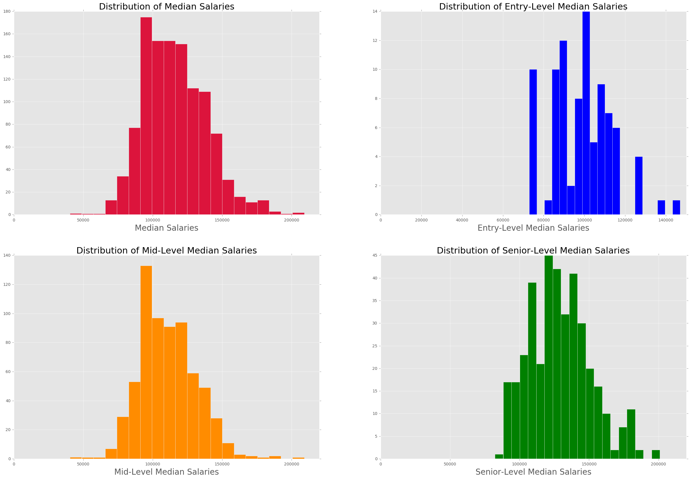
The distribution of entry-level, mid-level, and senior-level bins are: 90,663, and 378 respectively. The low sample size in entry-level bin compared to other bins is quite low, and will be problematic when plotting the distribution.

The image below shows the histogram for median salaries. There is skewness in the data, most likely due to high disparity in salaries in cities where cost of living is high, such as San Francisco and New York.

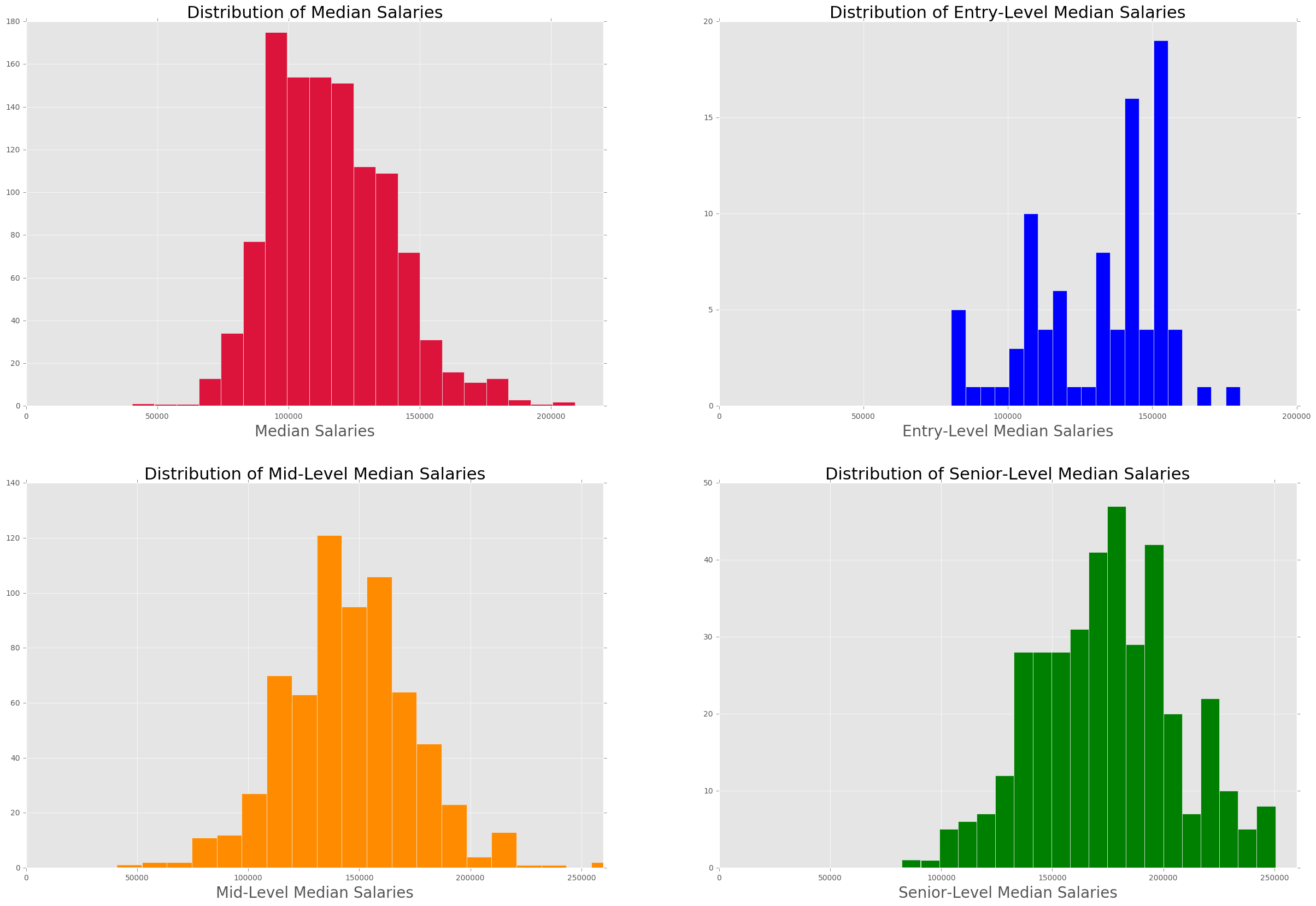
The image below shows the histogram for median salaries with cost of living factored in. The distributions show more of a normal distribution.

Assumptions

1) Normalizing salaries to adjust for Cost of Living, using NYC as base. 2) Used only experience, and cities as the features due not having access to skills in glassdoor. 3) There will be bias due to not having access to bonus or perks offered by companies. 4) Assumption is that each company in each market would offer similar bonus and perks, such that each company would pose an equal chance to hire a data scientist. In other words, they would be competitive in hiring for a data scientist.

Regression

Target Variable

• Above_median (1 if above median or 0 below median)

Features:

• Cities (Dummy for each City)
• Entry-level (Dummy)
• Mid-level (Dummy)
• Senior-level (Dummy)

Regression - Model 1

The cities used in this model were: Atlanta, Austin, Boston, Dallas, Detroit, Houston, Kansas City, Los Angeles, Minneapolis, Nashville, San Francisco, San Jose, and Washington DC.

GridsearchCV was used to find the optimal penalty and C value, using logistic regression as the estimator. GridsearchCV yielded: Penalty - L2, C - 0.9

The coefficients of the logistic regression are:

Variables	Coefficients
mid_bin	0.425147
senior_bin	2.796456
City_atlanta	1.383603
City_austin	1.996431
City_boston	0.539824
City_dallas	2.955003
City_detroit	5.770552
City_los angeles	1.783665
City_minneapolis	1.708747
City_nashville	1.434283
City_san francisco	0.031495
City_san jose	2.386696
City_seattle	0.941951
City_washington dc	-0.62814

Entry-level and New York were omitted to serve as the base case for their respective categories. Mid and Senior-level bins shows that we expect their probabilities to be above median is higher than entry-level Washington DC shows to have a negative coefficient meaning the probability of being the above median. This could be due to government jobs paying less due to having better benefits. One way to test for this, is to look at sectors and how each sector correlates to being above or below median.

Regression - Model 2

The cities used in this model were: Atlanta, Austin, Boston, Dallas, Detroit, Los Angeles, Minneapolis, Nashville, San Francisco, San Jose, and Washington DC.

Since the indeed dataframe does not contain Houston and Kansas City, these must be dropped from the glassdoor dataframe. From there, we perform the same regression as we used in the previous regression. 126 observations were dropped.

GridsearchCV yielded: Penalty - L2, C - 0.9, same as earlier.

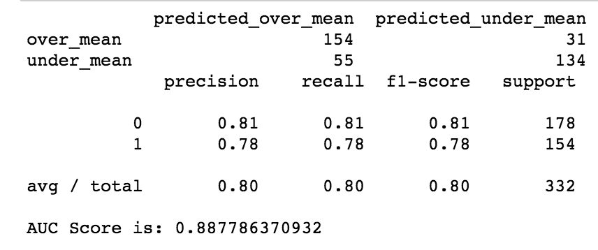
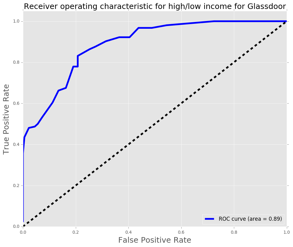
The AUC score increased by approximately 0.03, which shows that this model performs better. The F1 score increased from 0.77 to 0.80, which shows the model score increased.

Using this new model on the indeed dataframe as the test set, let’s see how well this model pridects salaries.

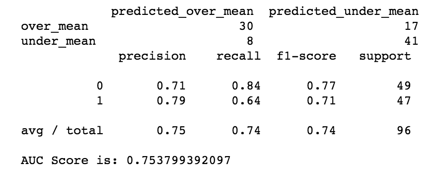
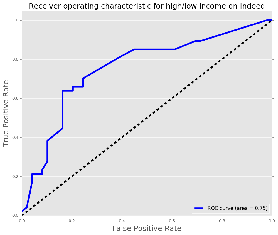
Conclusion

The model was used utilized GridsearchCV with logistic regression as the estimator. The target variable is whether the salary is above or below the median. The features used were cities (as dummies) and experience bins (entry-level, mid-level, and senior-level bins). The first regression had an AUC score of 0.86, while the second (after dropping Houston, and Kansas City since indeed dataframe did not have those cities) had an AUC score of 0.89. The AUC score increased 0.03, which is an improvement, the F1 score also increased by 0.03. With the features that were used, the model did a reasonable job in predicting whether a position would be above median or below median. Thus, using these features, the model should be robust during salary negotiations for potential data scientists.