Iowa Liquor Market Research for New Store Locations

Scenario involves a client, who is a liquor store owner in Iowa, that is looking to expand to new locations in Iowa. The data is available from the state of Iowa website. The 10% random sample of the data is availabe from here.. This study is part of a group project, involving myself, and two others, Amer Shalan and Thomas Voreyer.

The following steps are taken in this analysis:

1. Importing and loading Libraries
2. Tidying the Data/Data Munging
3. Exploratory Data Analysis & Visualization
4. Regression Analysis

To follow along, the Jupyter Notebook code can be found here.

The data set and external data sets can be found here.

Importing Dataset and Data Munging

The data set is 10% random sample of the 2015 State of Iowa liquor sales data. There were missing values, particularly in the County and Category fields. There were also Cities that were misspelled. The data set used is only for the year 2015. Once these were cleaned up, exploratory data analysis was performed.

Exploratory Data Analysis

The data is highly skewed (positively skewed) given the population density of Iowa is skewed. More populated areas had higher number of bottles sold, and also noticed that there were a small percentage of transactions that skewed the data, where bottles sold was greater than 100. Upon investigation, it was determined that restricting the data to bottles sold 25 and under would throw out a little under 4% of the data.

Plotting histograms of the the predictors that will be used later in the regression, like number of stores, show that the distribution is positively skewed as well.

Constructing the predictors

The target variable used in the regression is Bottles Sold per Store. The following predictors are used in the regression:

1. Unique Items per Store
2. Number of Stores per City
3. Avg Price (total sales / total bottles sold)
4. 2015 City Population
5. 2015 Yearly Per Capita Income per County

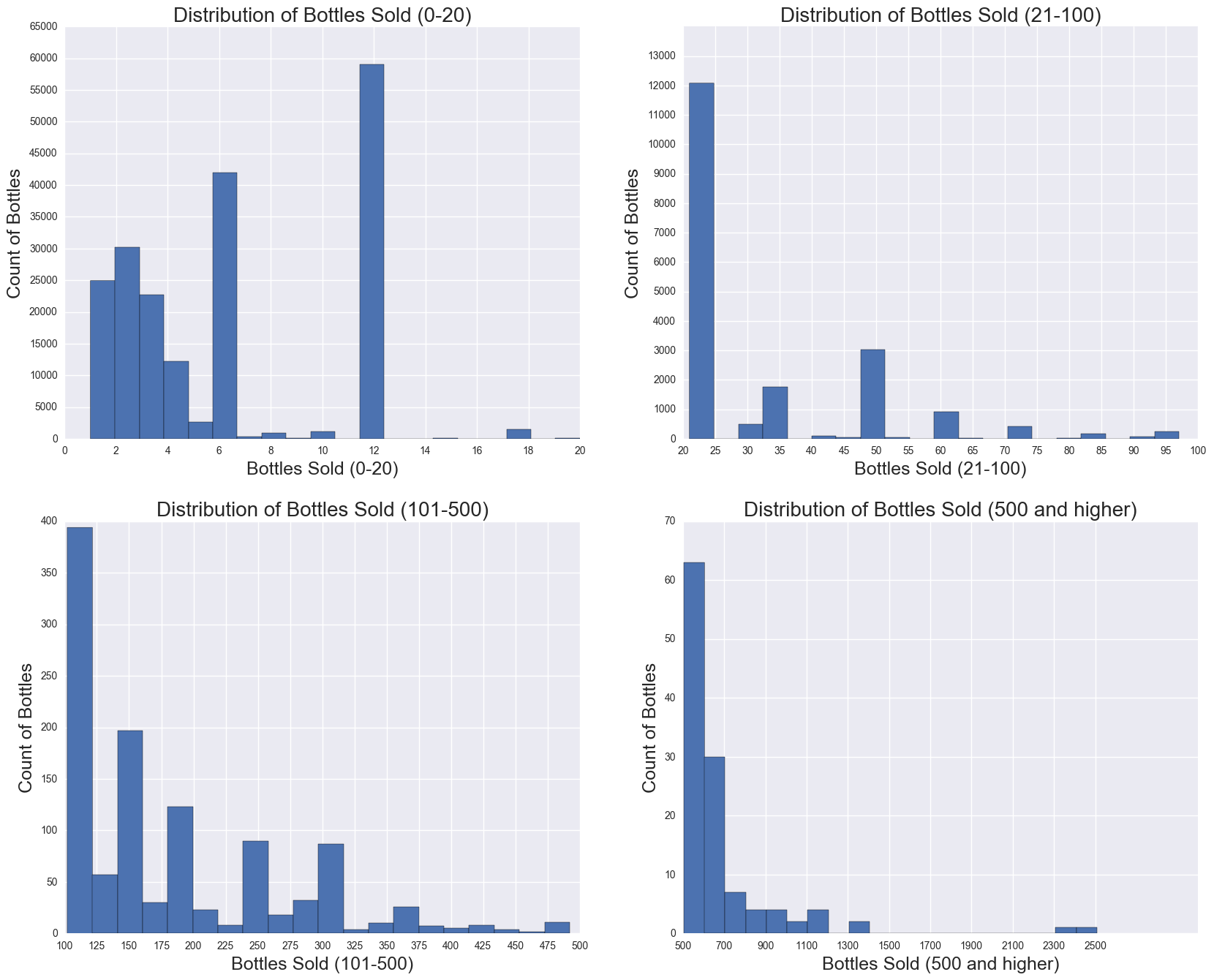
The target variable: Bottles Sold

Bottles Sold, which is the sum of all bottles sold per year per store number. The histogram, shown below, is broken down in groups of bottle sold. From the y-axis, it can be shown that the bottles sold is positively skewed. Histogram shows that 12 is the most frequent number, and that after 25, the count drops off significantly.

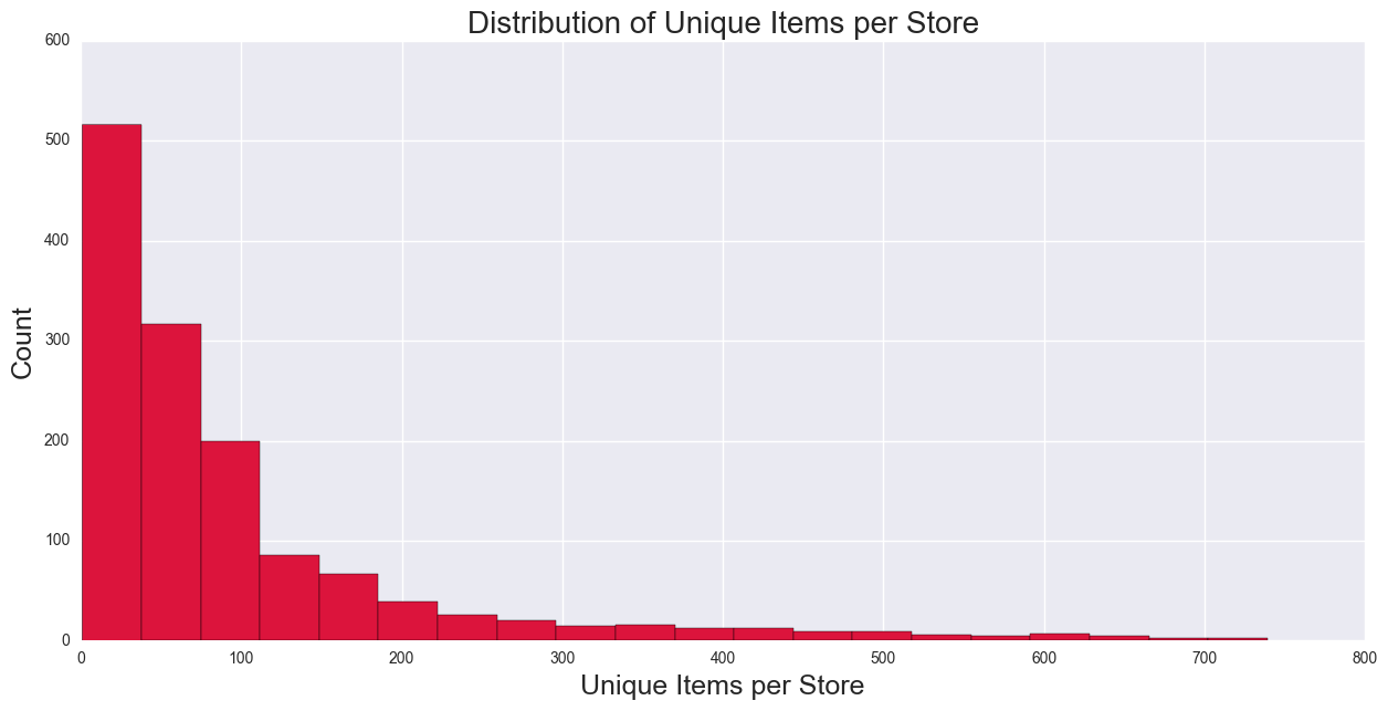
Unique Items per Store

This predictor looks at all unique items per store number and will be used as a proxy variable for store size. Hypothesis is that this predictor should be positively correlated with Bottles Sold, as the number of items available in a store, more goods to choose. Histogram below shows a positively skewed distribution.

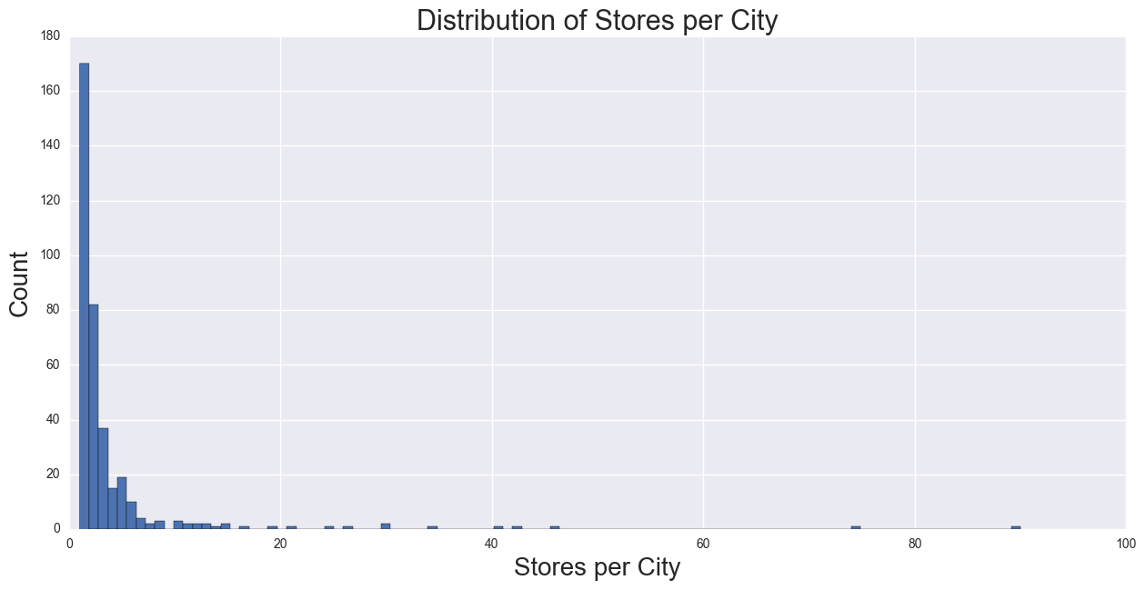
Number of Stores per City

Summing all the stores in a City gives Number of Stores per City, which is used as number of competitors in a city. This predictor should be negatively correlated with Bottles Sold, as the number of competition goes up, the higher the number consumers have to choose from, which means there should be a decrease in a store’s demand. Histogram shows the distribution as positively skewed.

Average Price

Aggregating total Sales (Dollars) and Bottle Sales, and taking an average of Sales/Bottles gives average price of the goods sold at each store. Price should be negatively correlated with Bottles Sold, as the demand curve should be a downward sloping curve.

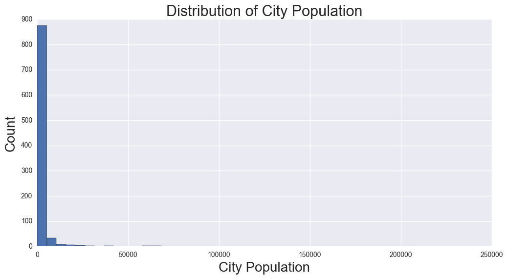
City Population

This external data is from the www.iowadatacenter.com website.

Per Capita Income

This external data is from the www.iowadatacenter.com website. Assumption is that liquor is a normal good, as when a income increases, demand increases, and falls as income decreases.

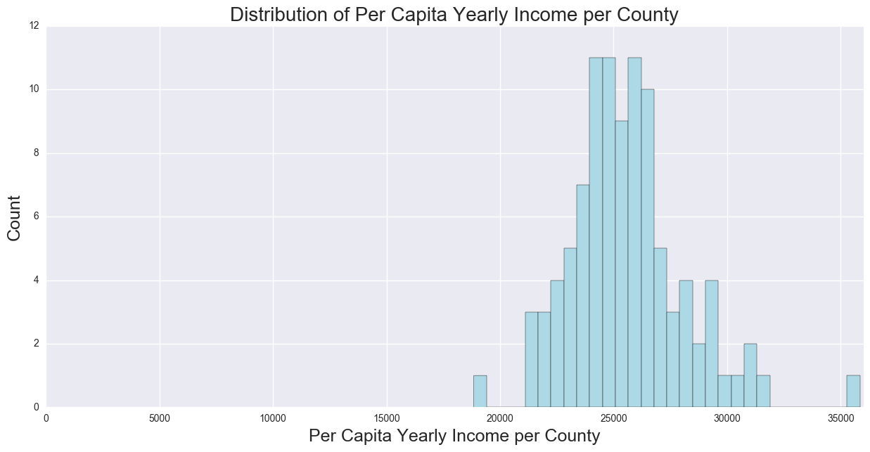
Both the Population and Per Capita Income should be positively correlated with Bottles Sales, as the number of people in a city as well as disposal income, the higher the demand for goods.

Regression Analysis

The dataframe will be constructed to get the target (df_y) and the data for the predictors (df_X), which will then be split into train and test sets. The target variable is Bottles Sold. The predictors that will be used are the following:

Target Variable:

• Yearly Bottles Sold (per each Store Number)

Predictors:

• Items per Store
• Average Price
• Stores per City
• Population
• Per Capita Yearly Income

Assumptions and Constraints:

• Constraining the data to bottles sold per transaction to 25 and under
• Each store in a city is competing against each other
• Log-normalization due to the skewness of the target and predictors
• Per Capital Yearly Income, which is for county, is uniform across cities in the county
• Liquor is a normal good, demand will increase as income increases and falls when income falls.

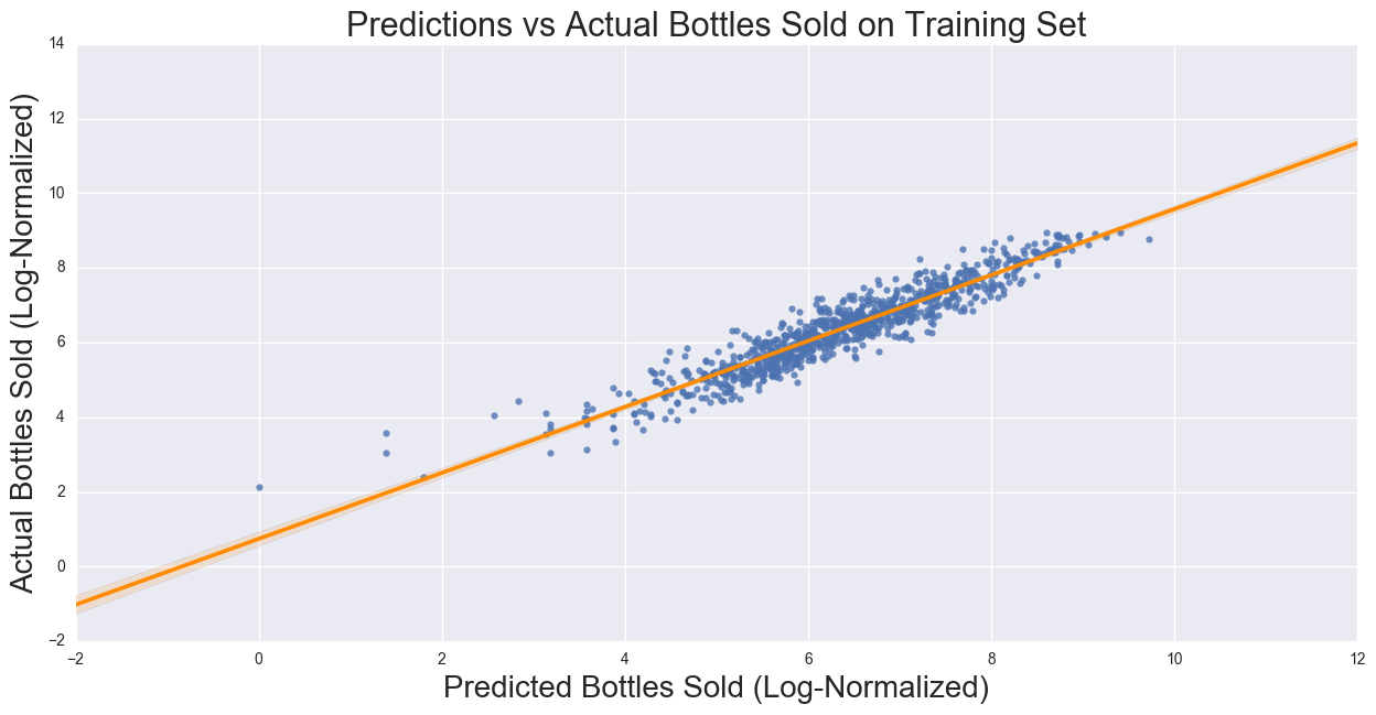
Linear Regression will be peformed on the training set, which will then be used to predict Bottles Sold. Before the regression is performed. Both the target and the predictors will be log-normalized because of the skewness, as shown in the histograms earlier.

Regression Results

R²:0.88 MSE: .168

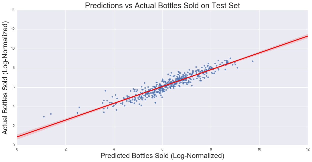
R²:0.87 MSE: .195

The model coefficients are:

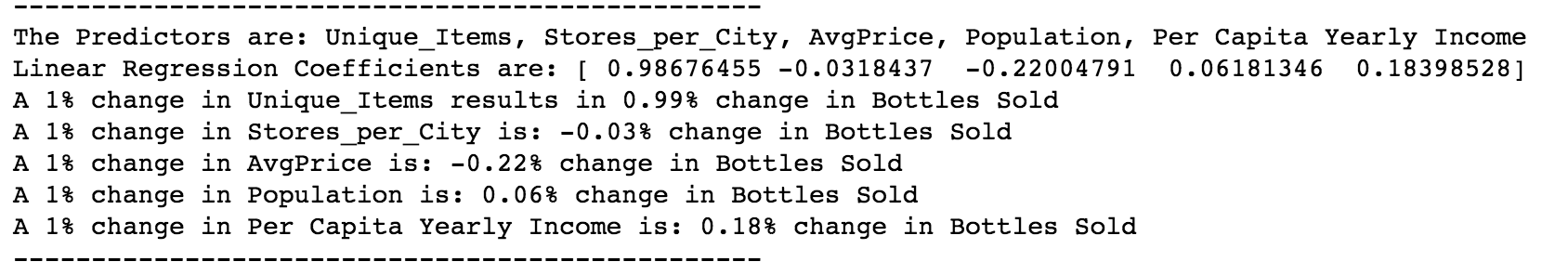
The correlation on the training dataset is 0.88, and the MSE is 0.16. The coefficients for the regression show the strongest predictor is Unique Items (positively correlated), followed by Average Price (negatively correlated), Stores per City/Number of competition (negatively correlated), and Population and Per Capital Yearly Income (both positively correlated). These relationships are what we expect to see: the number of items in a store would show that more available products to purchase, and as the number of competitors in the city as well as price should decrease the bottles sold. Population and Income should be positively correlated as the more people are in a city, the higher demand should be, and the more disposable income a person has, the more the person is able to spend on liquor. If the assumption of the Yearly per Capita Income is uniformly distributed across all cities in the county does not hold, then there would be a stronger bias, which requires city level Yearly per Capital Income.

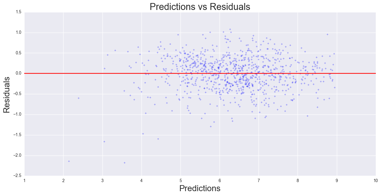
The correlation and MSE for the test data set are: 0.87 and 0.19,respectively. The model r-squared and MSE is approximately close to the same metrics in training set. Plotting predictions versus residuals shows that there is constant variance, thus, there is no systematic error in the model.

Forecasting a new entry

first method: What happens if another store enters the market? Assuming Quantity (Bottles Sold per City) and Avg Price does not change (also means Total Sales (Dollars) per city does not change), if we increased number of stores per city by 1, we can calculate the new AvgSales with entry of a new store. Sorting from highest to lowest, we find top 10 cities as consideration for markets to expand.

Once we know which markets to enter, we can find the average number of items among the competitors,types of competitors, and also the items and prices to which we place in the store.

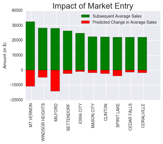
The following cities are either suburbs (Windsor Heights, Bettendorf, Coralville), college towns (Mt. Vernon, Iowa CityCedar Falls, or near a resort/lake (Spirit Lake, Milford, Mason City). Categorizing the Category Name to bins of liquor types, we can find the ideal mix of inventory using the average items per store, which was calculated above (164 items per store)

A second method was performed using Predicted Sales (Predicted Bottles Sold * Average Price - assumed constant). A new list of top 10 cities (predicted sales / n + 1) resulted in 7 of the 10 cities found in method 1.

The seven Cities that are in the list above:

• Windsor Heights
• Cedar Falls
• Milford
• Iowa City
• Mt. Vernon
• Mason City
• Coralville

Three new cities are in the top 10:

• Ames (college town)
• Monticello (rural iowa)
• Clear Lake (resort, next to Mason City)

These three weren’t in method 1 because the actual Sales were lower than the predicted, which means there was unobserved error that contributed to the high residuals between bottles sold and predicted bottles sold. These cities will not be considered in the possible new markets.

Given these two lists, it is recommended that these Cities be evaluated further for new location due to proximity colleges and distance to big cities:

• Windsor Heights (suburb of Des Moines, which is the capital and largest city)
• Cedar Falls (University of Northern Iowa and nex to Waterloo)
• Milford/Spirit Lake (a popular attraction during summer time)
• Iowa City/Coralville (University of Iowa is in Iowa City, Coralville is next to Iowa City)
• Mason City/Clear Lake (two cities next to each other, Clear Lake is a popular summer time attraction)

Evaluation went further into an ideal mix of types of liquor to be sold in the new location. By categorizing Category Name into several types ofliquor, we can conduct analysis on portfolio of placements in the new store.

Based on the mean of average unique items per city in top 10 cities in method 1 and the proportion of each type of liquor type sold of all 10 cities, the amount of each type of liquor can be estimated to be sold in the new location.

Proportion of liquor types sold in the top 10 cities:

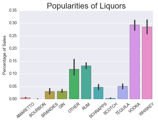
Applying the proportion of liquor types multiplied by the mean of average item per store (164 items) would result in the ideal mix:

Liquor Category	Ideal Mix (out of 164)
AMARETTO	1
BOURBON	0
BRANDIES	6
GIN	6
OTHER	18
RUM	21
SCHNAPPS	7
SCOTCH	1
TEQUILA	9
VODKA	49
WHISKEY	46

Conclusion

Given the 10% random sample of the Iowa Liquor Sales, the log-normalized Linear Regression Model was used to fit the data to the model. Using the yearly Bottles Sold per each store as the target variables, the predictors Unique Items per Store, Stores per City, Avg Price, Population, and Income were used to fit the model. The correlation and MSE of the data was 0.88 and 0.17, respectively. The model was then used to predict on the test set, and comparing actual Bottles Sold to predicted Bottles Sold, the correlation and MSE were 0.87 and 0.19, respectively.

Top 10 Cities are recommended using two methods: Actual Sales and Predicted Sales. Both methods involve Average Sales per number of competition, which is stores per city. Since we are interested in the scenario where a new store enters the market. We add 1 to the stores per city and divide Avg Sales by this number. Also assumed was that avg price and total bottles sold per city were constant. Taking the top 10 cities where the Avg Sales per store, the following cities are recommended for new markets for a new store location due to proximity to colleges and distances to major cities:

• Windsor Heights (suburb of Des Moines, which is the capital and largest city)
• Cedar Falls (University of Northern Iowa and nex to Waterloo)
• Milford/Spirit Lake (a popular attraction during summer time)
• Iowa City/Coralville (University of Iowa is in Iowa City, Coralville is next to Iowa City)
• Mason City/Clear Lake (two cities next to each other, Clear Lake is a popular summer time attraction)

Using the types of Liquor sold (binning them into types), the ideal mix of products to be sold was calculated, which is based on the aggregate of top 10 cities.

Further Analysis can be performed on the brands and size of each type of liquor, as well as the optimal price based on calculated price elasticities.