Evaluating Year 2000 Billboard Top 100 Data Set
Evaluation of the Year 2000 Billboard Data Set
The Year 2000 Billboard Data Set was analyzed as part of Project 2 for the General Assembly weekly Project. This dataset consists of 317 tracks that peaked in the Year 2000. Exploratory Data Analysis was performed with Python 2, Jupyter Notebook, Numpy,Pandas,matplotlib, and scipy. The process involved were the following: Loading the data set, Cleaning the Data, Exploratory Data Analysis/Visualization, and Hypothesis Testing. The Jupyter Notebook code can be found here.
The Hypothesis used in this analysis was to test to see if Pop genre had a different mean than the average during the Summer. The reason for this hypothesis is that Pop is generally thought to be more upbeat, and party type of songs that would be played in clubs, and other like events. The results will be discussed later. First, let’s discuss assumptions and risks. The following assumptions used in this analysis are the following: One genre per artist, the time field is the track length, which is converted to seconds. The genre field was cleaned up by going to Google and Wikipedia to verify the primary genre of the artist. For example, the original dataset had Madonna and Britney Spears listed as ‘Rock’, when they should be listed as ‘Pop’. The genre field was updated in a new column directly in the CSV via Microsoft Excel.
The risks in this analysis is that there is a potential crossover of genres, such as Destiny’s child, which could be thought of as ‘R&B’ and/or’ Pop’. There were approximately a little less than 5% of tracks that dropped off, came back, and then dropped off again in the charts. I will count those weeks in between as inactive weeks when counting total number of weeks in the charts. The data set only shows tracks that peaked in 2000, so it is only a subset of the tracks that were present in the Top 100 Billboard charts (by week). Let’s move on to the Data Munging.
Data Munging
The following steps were performed during data munging:
- Renaming Arist Column
- Converting date fields into Datetime objects
- Converting ‘time’ into seconds
- Replacing all ‘*’ with NaN
- Cleaning the ‘genre’ field
- Using pd.melt to get the ‘week’ columns by rows
- Dropping all NaN
Exploratory Data Analysis
There were two data sets used for exploratory data analysis: final, and final_bb. Final is the dataset where pd.melt was used to get weeks by rows. This allowed to use groupby to get a unique week which was used for the hypothesis testing. Final_bb is the original format of the billboard where there is a unique artist-track combination. The fields generated from the pd.melt process was used to join the final_bb data set through pd.merge.
The following graph shows the number of tracks by Month that were in the Billboard Top 100 for the tracks that peaked in 2000.
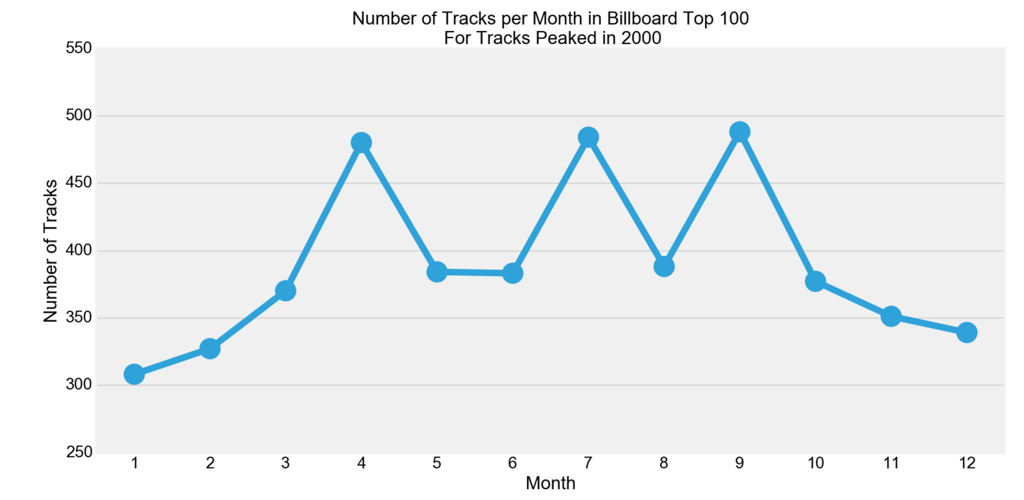
There seems to be peaks in April, July, and September. Let’s take a closer look for the Summer Season for Pop genre, since this is the focus of the hypothesis testing.
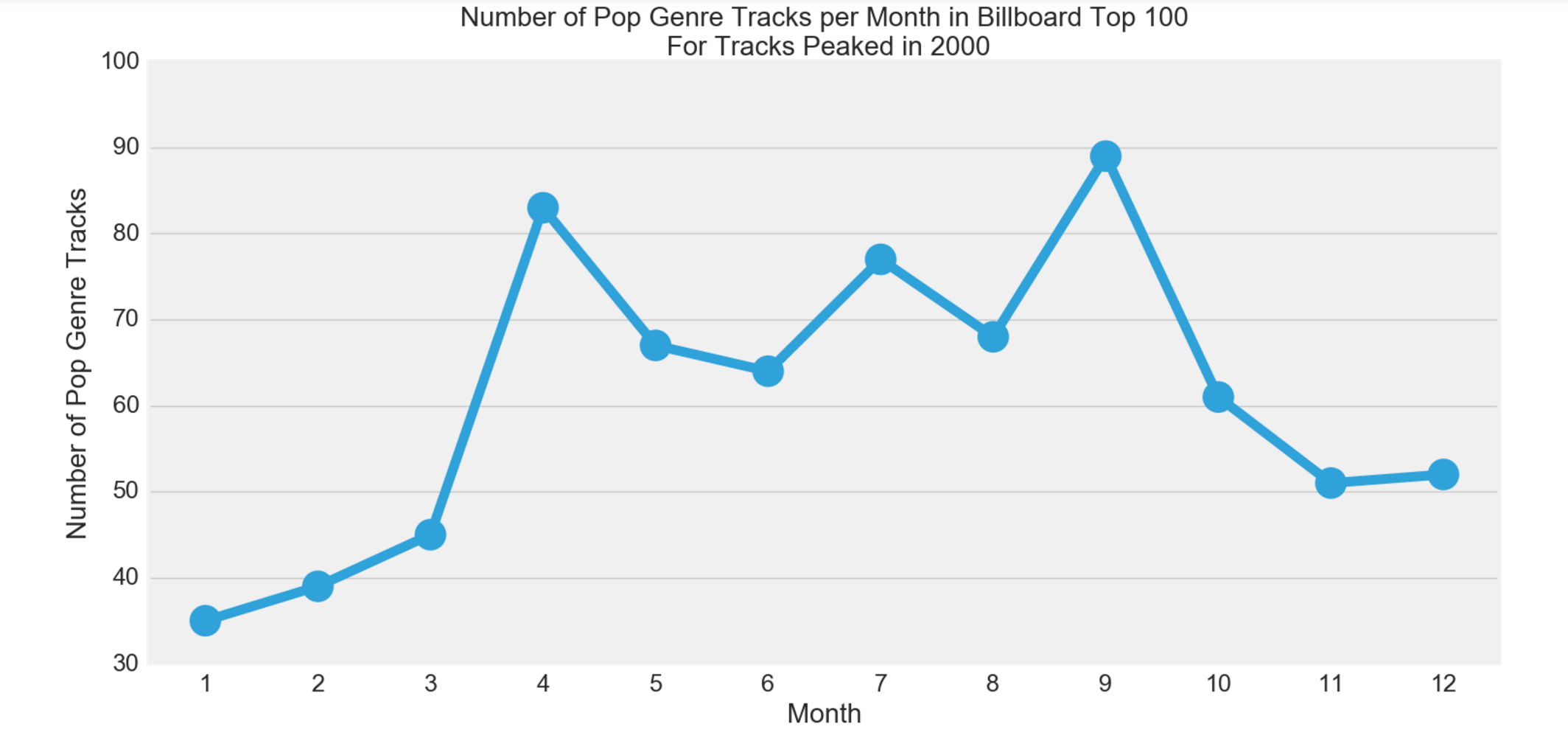
There seems to be in increase in the number of Pop genre tracks from April to September. Now, we shall test our hypothesis.
Hypothesis Testing
The null hypothesis is that there is no difference between the average position of Pop genre during the summer with the average position of a track in the Summer (regardless of Genre). The alternate hypothesis is that there is a difference. The final data set was used to perform this hypothesis by using a Boolean selection on season equal to summer, to test the mean Position, and then further on genre equal to Pop to test the Pop genre average position during the summer.
The model of the t-test (using scipy) was “stats.ttest_1samp(summer_pop,summer.mean())”, where summer_pop was the average position of all pop genre tracks in the summer, and summer.mean being the average position of all tracks in the summer. The result was that the test statistic was -3.93 and pvalue of 0.000115. Since the p-value is less than alpha of 0.5, we would reject the null hypothesis that there is no difference between the two means.
The two means of the sample were 50.6 for all tracks in the summer, and 42.4 for all pop genre tracks in the summer.
Conclusion
The results of the t-test lead us to reject the null hypothesis to that there is no difference between the two means. Of course, this is one of many hypothesis that could be conducted on this data set.
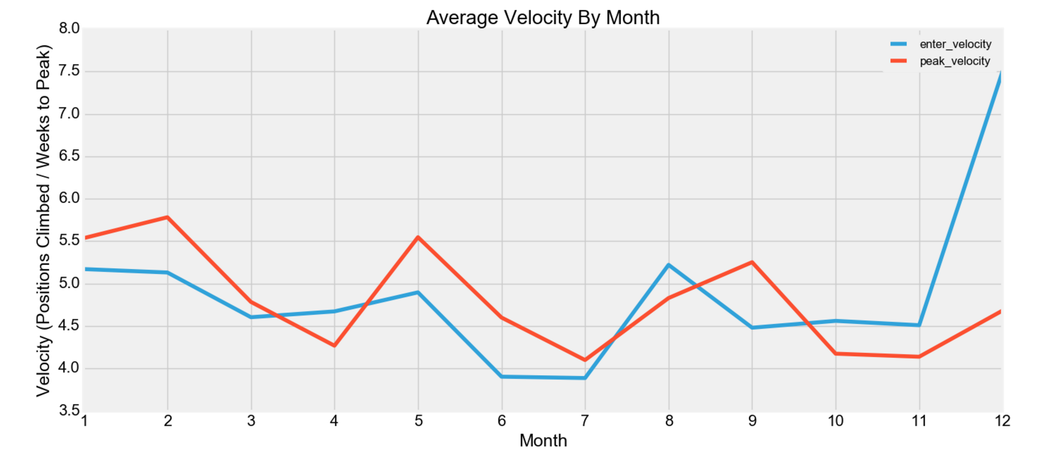
Another hypothesis could be that tracks increase faster (velocity) in the charts in the several weeks before Grammy’s (which is in February). Thus, December and January should see a higher increase. The chart below depicts that from November to December, there was a drastic increase in the velocity.